The study’s conclusions hinge on a surprising distinction: dogs don’t always tend to align with Earth’s magnetic field when they poop; they only tend to do it during times when the field’s direction is especially steadyThese steady conditions occurred about one fifth of the time in the study (table 8)..
If you’re familiar with the idea of p-hacking or data dredging, this kind of binning is probably enough to make you anxiousSee this xkcd cartoon for a fun take on the general concept, and this post for a criticism of this particular study along these lines., but I don’t want to focus on statistics today.
Instead, I want to highlight exactly how small these variations in the Earth’s magnetic field direction actually are, because I think the study’s authors took several steps to obscure this point.
In several recent posts, I have been exploring a way of doing trigonometry using vectors and their various products while de-emphasizing angle measures and trigonometric functions.
In this system, triangles are represented as sets of three vectors that add to 0
and rotations and reflections can be represented using geometric products of vectors. For vectors in the plane, the rotation of a vector v through the angle between vectors a and b can be represented by right multiplying by the product \hat{a}\hat{b}Reminder on notation: in these posts, lower case latin letters like a and b represent vectors, greek letters like \theta and \phi represent real numbers such as lengths or angles, and \hat{a} represents a unit vector directed along a, so that \hat{a}^2=1 and a = |a|\hat{a}. Juxtaposition of vectors represents their geometric product, so that ab is the geometric product between vectors a and b, and the geometric product is non-commutative, so the order of terms is important.
v_\mathrm{rot.} = v \hat{a}\hat{b}
and the reflection of v in any vector c can be represented as the “sandwich product”
v_\mathrm{refl.} = c v c^{-1} = \hat{c} v \hat{c}
Notice that none of these formulae make direct reference to any angle measures.
But without angle measures, won’t it be hard to state and prove theorems that are explicitly about angles?
Not really. Relationships between directions that can be represented by addition and subtraction of angle measures can be represented just as well using products and ratios of vectors with the geometric product. And the geometric product is better at representing reflections, which can sometimes provide fresh insights into familiar topics.
We’ll take as our example the inscribed angle theorem, because it is one of the simplest theorems about angles that doesn’t seem intuitively obvious (at least, it doesn’t seem obvious to me…).
In previous posts, I have shown how to visualize both the dot product and the wedge product of two vectors as parallelogram areas. In this post, I will show how the dot product and the wedge product are related through a third algebraic product: the geometric product. Along the way, we will see that the geometric product provides a simple way to algebraically model all of the major geometric relationships between vectors: rotations, reflections, and projections.
Before introducing the geometric product, let’s review the wedge and dot products and their interpretation in terms of parallelogram areas.
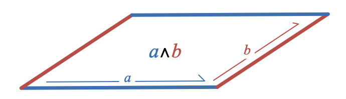
Given two vectors, a and b, their wedge product, a \wedge b, is straightforwardly visualized as the area of the parallelogram spanned by these vectors:
Recall that algebraically, the wedge product a \wedge b produces an object called a bivector that represents the size and direction (but not the shape or location) of a plane segment in a similar way that a vector represents the size and direction (but not the location) of a line segment.
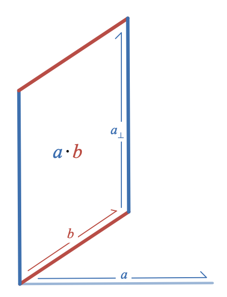
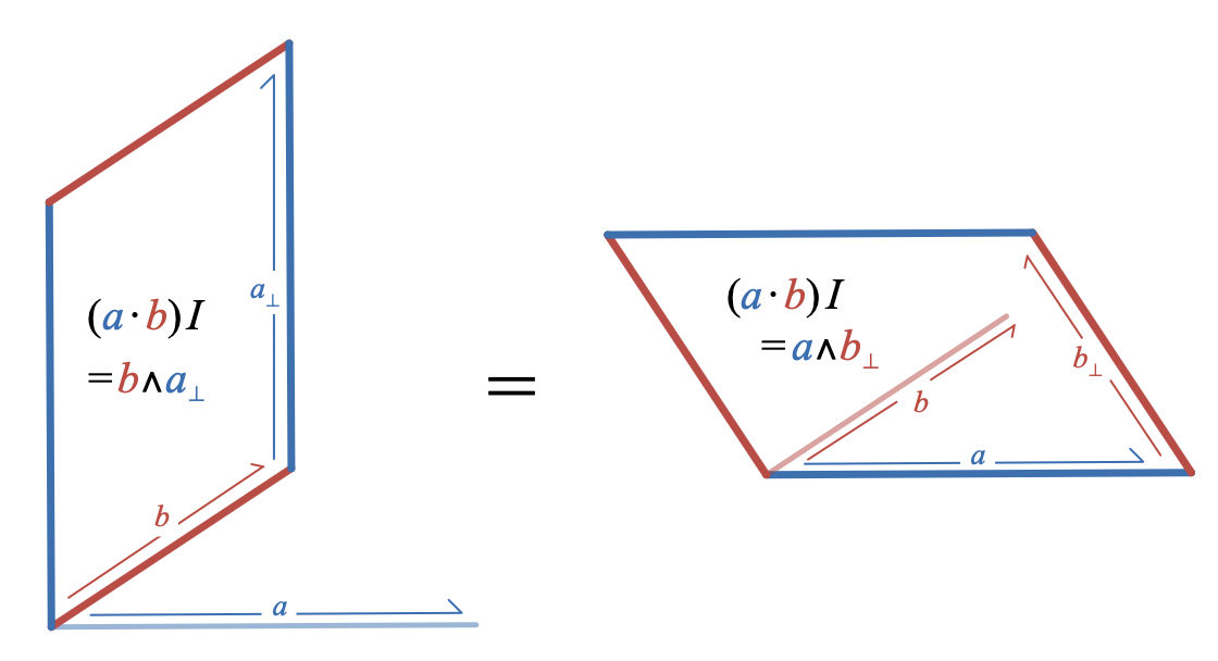
The dot product of the same two vectors, a \cdot b, can be visualized as a parallelogram formed by one of the vectors and a copy of the other that has been rotated by 90 degrees:
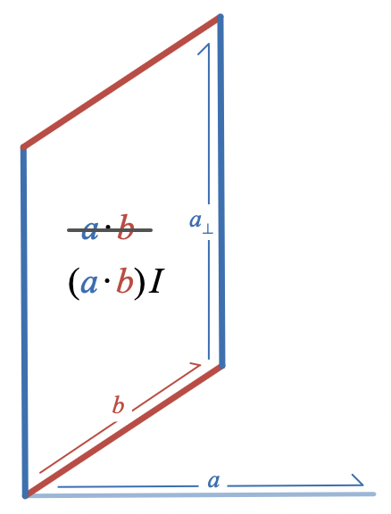
Well, almost. When I originally wrote about this area interpretation of the dot product, I didn’t want to get into a discussion of bivectors, but once you have the concept of bivector as directed plane segment, it’s best to say that what this parallelogram depicts is not quite the dot product, a \cdot b, which is a scalar (real number), but rather the bivector (a \cdot b) I where I is a unit bivector.
The scalar a \cdot bscales the unit bivector I to produce a bivector with magnitude/area a \cdot b. It’s hard to draw a scalar on a piece of paper without some version of this trick. Once you’re looking for it, you’ll see that graphical depictions of real numbers/scalars almost always show how they scale some reference object. It could be a unit segment of an axis or a scale bar; here it is instead a unit area I.
Examining the way that the dot product and the wedge product can be represented by parallelograms suggests an algebraic relationship between them:
(a \cdot b) I = b \wedge a_\perp
where a_\perp represents the result of rotating a by 90 degrees. Since the dot product is symmetric, we also have
(a \cdot b) I = a \wedge b_\perp
To really understand this relationship, we’ll need an algebraic way to represent how a_\perp is related to a; in other words, we’ll need to figure out how to represent rotations algebraically.
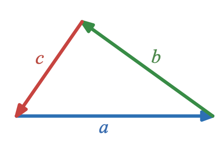
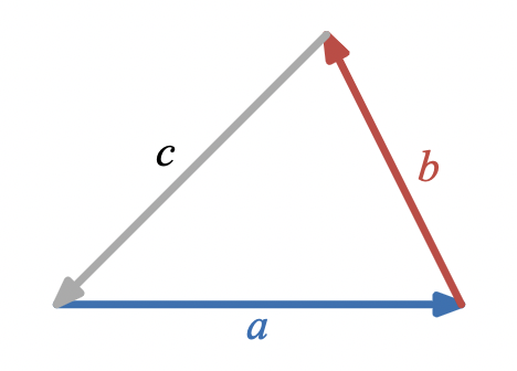
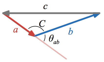
A visual way of expressing that three vectors, a, b, and c, form a triangle is
and an algebraic way is
a + b + c = 0
In a previous post, I showed how to generate the law of cosines from this vector equation—solve for c and square both sides—and that this simplifies to the Pythagorean theorem when two of the vectors are perpendicular.
In this post, I’ll show a similarly simple algebraic route to the law of sines.
In understanding the law of cosines, the dot product of two vectors, a \cdot b, played an important role. In understanding the law of sines, the wedge product of two vectors, a \wedge b, will play a similarly important role.
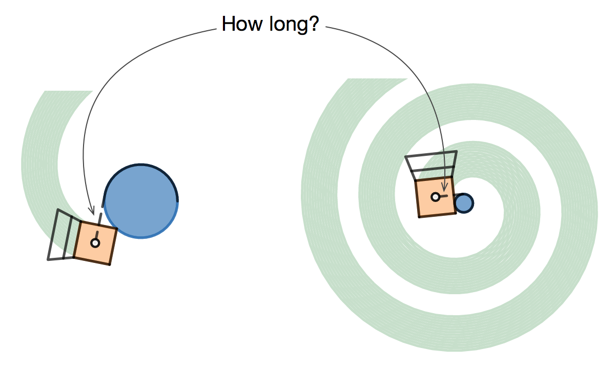
I recently posted a geometry puzzle about an autonomous lawn mower steered by a rope and a peg. How much rope remains unspooled from the peg when the mower collides with it? If you haven’t seen the puzzle yet, go check out last week’s post and give it a try.
One of the joys of being an engineer at Desmos is that my collaborators occasionally bring me math problems that they need to solve to make something that they’re building work right. I love tricky little geometry problems, and I’d solve them as a hobby if they weren’t part of my job. When it helps our team get on with the work, so much the better.
In today’s post, I’d like to share one of these puzzles that came up while building Lawnmower Math, and invite you to solve it yourself.
I have a confession to make: I have always found symbolic algebra more intuitive than geometric pictures. I think you’re supposed to feel the opposite way, and I greatly admire people who think and communicate in pictures, but for me, it’s usually a struggle.
For example, I have seen many pictorial “proofs without words” of the Pythagorean Theorem. I find some of them to be quite beautiful, but I also often find them difficult to unpack, and I never really think “oh, I could have come up with that myself.”
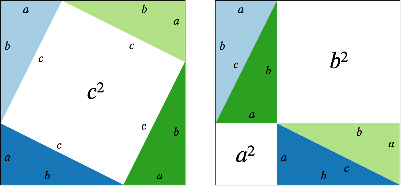
I like this proof a lot. It’s fairly simple to interpret (more so than some of the other examples in the genre), and quite convincing. We have
c^2 = a^2 + b^2
because, along with the same four copies of a triangle, both sides of this equation fill up an identical area.
Even so, it’s odd to me that this diagram involves four copies of the triangle. This is one of those “I couldn’t have come up with this myself” stumbling blocks.
For comparison, I’ll give an algebraic proofHere and throughout I am using the word “proof” quite loosely. Forgive me, I am a physicist, not a mathematician. of the Pythagorean theorem using vectors. The condition that three vectors a, b, and c traverse a triangle is that their sum is zero:
a + b + c = 0
Solving for c gives
c = -(a+b)
and then dotting each side with itself and distributing gives
\begin{aligned}
c \cdot c &= \left(a+b\right) \cdot \left(a + b\right) \\
&= a \cdot a + a \cdot b + b \cdot a + b \cdot b \\
&= a^2 + b^2 + 2 a \cdot b
\end{aligned}
The condition that vectors a and b form a right angle is just that a \cdot b = 0, and in that special case, we have the Pythagorean theorem:
c^2 = a^2 + b^2
The thing I like about this algebraic manipulation is that it is a straightforward application of simple rules in sequence. There are dozens of ways to arrange 4 congruent triangles on a page (probably much more than dozens, really), but the algebra feels almost inevitableIt does take practice to get a feel for which rules to apply to achieve a given goal, but there are really only a few rules to try: distributivity, commutativity, associativity, linearity over scalar multiplication, and that’s about it..
Write down the algebraic condition that vectors forming the sides of any triangle must satisfy.
We’re interested in a function of one of the side vectors, c^2, so we solve for c and apply the function to both sides.
We transform the right hand side by applying distributivity of the dot product across addition, and commutativity of the dot product, i.e. a \cdot b = b \cdot a.
Right triangles in particular are a simplifying special case where one term drops out.
I also think it’s important that the algebraic manipulation embeds the Pythagorean theorem as a special case of a relationship that holds for all triangles: the Law of CosinesThe following diagram shows the relationship between the vector form of the law of cosines, c^2 = a^2 + b^2 + 2 a \cdot b, and the angle form of the law of cosines, c^2 = a^2 + b^2 - 2 |a||b|\cos C In the angle form, C is an interior angle, but in the vector form, if a \cdot b = |a||b|\cos(\theta_{ab}), then \theta_{ab} is an exterior angle. This is the origin of the difference in sign of the final term between the two forms.. If you have a theorem about right triangles, then you’d really like to know whether it’s ever true for non-right triangles, and how exactly it breaks down in cases where it isn’t true. Perhaps there’s a good way to deform Pythagoras’ picture to illustrate the law of cosines, but I don’t believe I’ve seen it.
For these reasons, I’ve generally been satisfied with the algebraic way of thinking about the Pythagorean theorem. So satisfied, I recently realized, that I’ve barely even tried to think about what pictures would “naturally” illustrate the algebraic manipulation.
In the remainder of this post, I plan to remedy this complacency.
Robert Vanderbei has written a beautifulseries of articles and talks about a method for finding the radius of the earth based on a single photograph of a sunset over a large, calm lake.
Vanderbei’s analysis is an elegant and subtle exercise in classical trigonometry. In this post, I would like to present an alternative analysis in a different language: Geometric Algebra. I believe that geometric algebra is a more powerful system for formulating and solving trigonometry problems than the classical “lengths and angles” approach, and it deserves to be better known. Vanderbei’s sunset problem is simple to understand and challenging to solve, so it makes a nice benchmark.
Here’s Vanderbei’s sunset problem. If the earth was flat, photographs of the sun setting over water would look like this:
Notice that the reflection dips just as far below the horizon as the sun peaks above it.
Actual photographs of the sun setting over calm water (like Vanderbei’sUpdate: I should have been more careful to note that most photographs of sunsets over water actually don’t look like Vanderbei’s photograph (or my diagram) because of waves and atmospheric effects, and that sensor saturation artifacts make it hard to interpret images like this. Reproducing Vanderbei’s image may be somewhere between hard and impossible. More Below.) look more like this:
Kakuro is a number puzzle that is a bit like a combination between Sudoku and a crossword puzzle. Imagine a crossword puzzle where, instead of words, blocks of boxes are filled with combinations of digits between 1 and 9, and instead of clues about words, you are given sums that a block of digits must add up to.
When you’re solving a Kakuro puzzle, it’s helpful to be able to generate all the combinations of m different digits that add up to a given sum. A recent thread on the julia-users mailing list considered how to implement this task efficiently on a computer.
In this post, I’d like to show a progression of a few different implementations of the solution of this same problem. I think the progression shows off one of Julia’s core strengths: in a single language, you are free to think in either a high level way that is close to your problem domain and easy to prototype, or a low level way that pays more attention to the details of efficient machine execution. I don’t know any other system that even comes close to making it as easy to switch back and forth between these modes as Julia does.
Attention Conservation Notice: If you’re looking for information on how to solve Kakuro with a computer, you should probably look elsewhere. This post is a deep dive into a tiny, tiny subproblem. On the other hand, I’ll show how to speed up the solution of this tiny, tiny subproblem by a factor of either ten thousand or a million, depending how you count, so if that sounds fun you’re in the right place.
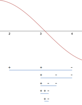
Bisection is about the simplest algorithm there is for isolating a root of a continuous function:
Start with an interval such that the function takes on oppositely signed values on the endpoints.
Split the interval at its midpoint.
Recurse into whichever half has endpoints on which the function takes on oppositely signed values.
After each step, the new interval is half as large as the previous interval and still contains at least one zero (by the Intermediate Value Theorem).
I want to highlight a couple of interesting issues that arise when implementing bisection in floating point arithmetic that you might miss if you just looked at the definition of the algorithm.
 In the angle form,

