Sunset Geometry

Robert Vanderbei has written a beautiful series of articles and talks about a method for finding the radius of the earth based on a single photograph of a sunset over a large, calm lake.

Vanderbei’s analysis is an elegant and subtle exercise in classical trigonometry. In this post, I would like to present an alternative analysis in a different language: Geometric Algebra. I believe that geometric algebra is a more powerful system for formulating and solving trigonometry problems than the classical “lengths and angles” approach, and it deserves to be better known. Vanderbei’s sunset problem is simple to understand and challenging to solve, so it makes a nice benchmark.

Here’s Vanderbei’s sunset problem. If the earth was flat, photographs of the sun setting over water would look like this:

Notice that the reflection dips just as far below the horizon as the sun peaks above it.

Actual photographs of the sun setting over calm water (like Vanderbei’s^⊕Update: I should have been more careful to note that most photographs of sunsets over water actually don’t look like Vanderbei’s photograph (or my diagram) because of waves and atmospheric effects, and that sensor saturation artifacts make it hard to interpret images like this. Reproducing Vanderbei’s image may be somewhere between hard and impossible. More Below.) look more like this:

Notice the shortened reflection. This happens because of the curvature of the earth, and by measuring the size of this effect, it is possible to infer the ratio of the earth’s radius to the camera’s height above the water^⊕The main virtue of Vanderbei’s method is that the evidence is so directly visual (and that you can collect it with a smart phone on vacation). If you want to make a simpler and better measurement with a similar flavor, climb a mountain and use an astrolabe; the math is simpler and the measurement will be more accurate..

Vanderbei calls the angle of the sun above the horizon \alpha, and the angle of the sun’s reflection below the horizon \beta. With geometric algebra at our disposal, it’s often algebraically simpler to work with unit directions than angles, so I will also label unit directions from the camera to the top of the sun, s, the horizon, t, and the bottom of the sun’s reflection from the water, w.

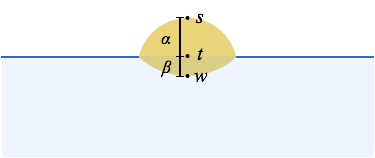
To analyze this problem, it’s helpful to consider a side view:

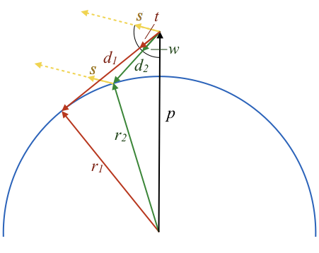
There are two important triangles in this diagram: the triangle formed by the center of the earth, the camera, and the horizon (drawn in red), and the triangle formed by the center of the earth, the camera, and the reflection point where the top of the sun reflects off the water (drawn in green).

The triangle equations

Triangles have a very simple algebraic representation in terms of vectors^⊕In this post, I am following the common geometric algebra convention of writing vectors as plain, lower-case letters, and using Greek letters for scalars. This takes a little getting used to if you are accustomed to bold face or over-arrows for vectors, but skipping all the decorations makes it simpler to work with lots of vectors.:

These simple sums of vectors subsume all the information about the relationships of lengths and angles that is expressed in classical trigonometry through “soh-cah-toa”, the triangle postulate (sum of interior angles is 180 degrees), the Pythagorean theorem, and the laws of cosines and sines. Quite an improvement.

It will be useful to re-express d_1 and d_2 in terms of the unit directions defined previously in order to relate other vectors to known directions:

(1a)

(1b)

In other words, d_1 is directed toward the horizon, and d_2 is directed toward the bottom of the reflection from the water.

Besides these triangles, there are a few salient geometric facts:

The horizon condition

The line of sight to the horizon is tangent to the earth at the horizon, and is therefore perpendicular to the radius of the earth through the horizon.

(2)

The reflection condition

In terms of angles, this is expressed as “angle of incidence equals angle of reflection”. In terms of vectors, it can be restated as

or

(3)

Known lengths

We know the lengths of some of these vectors in terms of the earth’s radius, \rho, and the height of the camera above the shoreline, \delta,

(4a)

(4b)

(4c)

Squaring both sides of the first triangle equation (1a), and using the horizon condition (2) (or equivalently, using the Pythagorean theorem) also allows finding the length of d_1:

(4d)

Equations (1-4) contain all of the geometrical information^⊕I assumed one other important piece of geometrical information by writting “s” in two places on the side-view diagram. This corresponds to the (excellent) approximation that the sun is very far away compared to other lengths. needed to solve algebraically for the Earth’s radius, \rho, in terms of the given angles/directions (\alpha and \beta, or s, w, and t) and the height of the camera above the shoreline, \delta.

Introducing Geometric Algebra

So far, I have formulated everything in terms of vector algebra that should look familiar to students of physics or engineering (Gibbs vector algebra). To actually solve the equations, I will use a few additional notions from geometric algebra.

Geometric algebra is the answer to the question “what if I could multiply and divide by vectors?” It introduces a new associative (but non-commutative) invertible product between vectors: the geometric product. The geometric product between vectors a and b is simply written ab. The geometric product of a vector with itself equals a scalar (the square of the length of the vector),

This fact, combined with associativity and the other familiar rules for multiplication, is enough to define the geometric product uniquely.

The symmetric and anti-symmetric parts of the geometric product have important geometric meaning, and are traditionally given their own special symbols^⊕Physicists may be mystified to realize that, based on this definition of the geometric product, parallel vectors commute, and perpendicular vectors anti-commute. What else does that remind you of?:

I will assume that the dot product, a \cdot b, is familiar: it is related to the projection of one vector onto another, and proportional to the cosine of the angle between them.

The wedge product, a \wedge b, is probably only familiar if you have studied differential forms (or geometric algebra, of course), but it is very similar to the more familiar cross product, a \times b. It represents the directed area of the parallelogram spanned by two vectors, and is proportional to the sine of the angle between them^⊕Anti-symmetry and bi-linearity are exactly what is needed to represent area: a vector spans no area with itself (anti-symmetry), and the area of a parallelogram scales linearly with the lengths of each of its legs (bi-linearity).

The wedge product is extremely useful in linear algebra because it represents linear subspaces spanned by any number of vectors in a way that can be manipulated algebraically.. Whereas the cross product represents directed area by a vector orthogonal to the area (a trick that works only in 3 dimensions), the wedge product represents a directed area by a different kind of object called a "bivector." The wedge product is associative (like the geometric product, but unlike the cross or dot products), and the wedge product of more than two vectors builds objects of higher "grades." The wedge product between 3 vectors is a trivector representing a directed volume (of the parallelepiped spanned by them), and the wedge product between k different vectors is a k-vector representing a directed k-dimensional volume (which is always zero in spaces of dimension less than k).

We can turn these definitions around to write the geometric product in terms of the dot and wedge products,

where \left\langle a b \right\rangle_0 and \left\langle a b \right\rangle_2 are notations for “the scalar part” and “the bivector part”.

There is a strange thing about this object: it represents the sum of two different “kinds of things,” a scalar and a bivector. But this should be no more troubling than the fact that a complex number represents the sum of a “real number” and an “imaginary number,” (in fact, there is an extremely close relationship between complex numbers and the geometric product of two vectors). With experience, it becomes clear that a sum of a scalar and a bivector is exactly what is needed to represent the product of two vectors in an associative, invertible way.

The geometric product gives us two new super powers when working with vector equations:

Solving equations involving products of vectors.

Given an equation for two different products of vectors

if b is known, we can solve for a by right-multiplying by b^{-1} (i.e. dividing by b).

b^{-1} is well-defined by demanding

left-multiplying by b

and dividing through by the scalar b^2

Contrast this to the dot product and the cross/wedge product. In general, even when b is known, it is not possible to uniquely solve any one of the following equations for a.

The first equation only determines the part of a that is parallel to b, and the second two equations only determine the part of a that is perpendicular to b. You need both of these to solve for all of a, and that’s what the single geometric product gives you.

Transitive relationships between vectors

It frequently occurs that we know the relationships of two vectors a and b to a third vector c, and we would like to use this information to determine the relationship between a and b. Algebraically, we can take the unknown product

and insert the identity

between the factors and re-associate

thus re-expressing the unknown product ab in terms of the known products products ac and cb.

Because cc^{-1} = 1, we can insert it anywhere that it’s convenient in any product of vectors. This has the same practical effect as resolving vectors into parts parallel and perpendicular to c. This is an example of a very general technique that shows up in many forms throughout mathematics: inserting an identity to resolve a product into simpler pieces.

We will use this trick twice below at a critical moment in solving the sunset problem.

Reformulating the horizon and reflection conditions

In order to make efficient use of geometric algebra’s tools, it is useful to reformulate equations (2) and (3) (the horizon and reflection conditions) in terms of the geometric product instead of the dot product.

Horizon condition

Consider the geometric product

where the first equality is an expression of the general vector identity ab = a \cdot b + a \wedge b, and the second equality follows from r_1 \cdot t = 0, our previous form of the horizon condition (2).

In two dimensions, there is only one unit bivector, called I, spanned by any two orthogonal unit vectors e_1 and e_2:

Therefore r_1 \wedge t is proportional to I, and since r_1 and t are orthogonal, we can write

(2’)

Reflection Condition

Our previous version of the reflection condition (3) also has the form of an orthogonality condition:

so, similarly to the way we rewrote the horizon condition, we can rewrite this in terms of the geometric product as ^⊕There’s another way to write reflections in geometric algebra that shows up more commonly: r_2 s = - w r_2 or s = - r_2^{-1} w r_2 = - r_2 w r_2^{-1} .

This other form is very useful for composing reflections into rotations, or factoring rotations into reflections, but the form we use here involving forming an orthogonal vector will be more convenient when it comes time to solve for r_2.

It will simplify later algebra to define a new unit vector based on this equation:

so that the reflection condition becomes

(3’)

Solving for the Earth’s radius

Now that we have rewritten our main geometric conditions in terms of the geometric product instead of the dot product, we are ready to solve the triangle equations.

First, eliminate p and set the left hand sides of (1a) and (1b) equal to one another^⊕This equation involving a sum of four vectors is a “quadrilateral equation” in exactly the same sense as our earlier triangle equations: it expresses the fact that the red vectors and green vectors in our diagram form a quadrilateral.:

The magnitude |d_2| is unknown, so we could proceed by solving for it, but it is more efficient to simply eliminate it in the following way. First, multiply both sides of the equation on the right by w:

Now we can use “grade separation” to separately consider the scalar and bivector parts of this equation. Since w^2 is a scalar, the |d_2| dependence drops out of the bivector part:

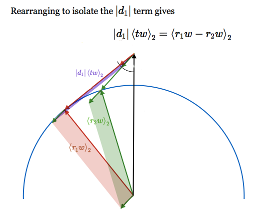
Rearranging to isolate the |d_1| term gives

We can now take advantage of the horizon and reflection conditions to rewrite the unknown products r_1 w and r_2 w in terms of known products by inserting factors of t t = 1 and g g = 1 and re-associating (this is the second “super power” from the introduction above):

We can simplify both r_1 t and r_2 g to \rho I using the horizon (2’) and reflection (3’) conditions:

Now expanding the geometric products of vectors into dot and wedge product gives

where I have dropped terms like \left\langle t \cdot w\right\rangle_2 = 0 and \left\langle I (t \wedge w - g \wedge w)\right\rangle_2 = 0 because they contain no part with grade 2.

We can take advantage of the known length |d_1|^2 derived as (4d) by taking the magnitude squared of both sides:

To simplify further algebra, for the term in brackets, introduce

which is written entirely in terms of known products of directions. This gives

Now substituting from (4d) for |d_1|^2 gives

and dividing through by \rho^2 gives

and finally, we are able to solve for \rho, the radius of the earth^⊕I (and Vanderbei) have chosen a positive square root here. What, if anything, does the negative square root represent?

(5)

We can recover Vanderbei’s final answer by rewriting \epsilon^2 in terms of angles using the following relationships:

so

\epsilon^2 = \frac{\left(\cos(\gamma) - \cos(\beta)\right)^2}{\sin(\beta)^2}

From this and (5), it is a simple exercise in trigonometric identities to recover the form given on slide 28 in Vanderbei’s talk, but there are two better forms that I will show instead.

First, a small angle form.

Using the general approximations

we can simplify (5) to

(5’)

The angles in Vanderbei’s photo are quite small, so this approximation is accurate to better than one part in a million^⊕It’s also simpler than other small angle approximations previously given by Vanderbei.. Since the uncertainty in the angles and camera height are about 10% each, this small angle approximation is certainly sufficient.

In fact, when calculating with rounded (floating point) arithmetic, the small angle form (5’) is actually more accurate than the exact form given by Vanderbei. This counterintuitive fact occurs because the exact form suffers from “catastrophic cancellation,” the result of subtracting approximately equal values that have been computed with rounding error.

We can get rid of one place such cancellation occurs by multiplying the numerator and denominator of our exact expression (5) by 1 + \sqrt{1 + \epsilon^2} to get

(5’’)

and we can get rid of another source of cancelation by replacing the difference of cosines in our expression for \epsilon^2 with a difference of sines using the general trigonometric identity^⊕This identity is related to the classical Haversine Formula from spherical trigonometry. Evelyn Lamb has written a wonderful blog post on this and other creatures in the zoo of forgotten trigonometry functions.

so that:

This is helpful because we’re now subtracting two numbers that are very close to 0 instead of very close to 1, and intermediate rounding to a fixed number of digits throws away less information for numbers that are close to 0 than for numbers that are close to 1.

Plugging this expression for \epsilon^2 into the non-cancelling form for \rho (5’’) now allows computing \rho without undue rounding issues.

To evaluate \rho in terms of measured parameters, insert the following values into either (5’) or (5’’)

This is 20% larger than the true value, 3960 mi^⊕It’s also different in the second digit from the answer given by Vanderbei (slide 28). I think this is attributable to the “catastrophic cancellation” discussed above, combined with low precision calculation.. Not too bad.

Comparison to other systems

Classical trigonometry

At this point, perhaps you are thinking that I’m crazy to believe that the analysis above is simpler than doing classical trigonometry. We learned trigonometry in high school, and it wasn’t all that hard, right? And the geometric algebra analysis involves a bunch of unfamiliar notations, keeping track of non-commuting multiplications, and the new geometric notion of “bivector^⊕On the other hand, it does give you algebraic super powers..”

But the classical trigonometry analysis of this problem is hard. Harder than the trigonometry problems that you solved in high school. If you don’t believe me, take a crack at solving it without referring to Vanderbei’s analysis. Or even just follow along with the talk and fill in all the algebra.

The subtlest part of Vanderbei’s formulation of the problem involves noticing a non-trivial relationship between 4 angles:

and the subtlest part of solving the problem involves solving the trigonometric equation^⊕This equation is transcendental in the angles, but turns out to be algebraic (quadratic) in \cos(\phi).

for \cos(\phi).

Solving difficult trigonometry problems in the classical language tends to involve constantly moving back and forth between algebraic expressions and the diagrams. This is because the full relationships between lengths and angles as separate entities are much more complicated than the relationships between vectors, which keep information about magnitude and direction conveniently integrated together. For this reason, in classical analyses, much of the information about lengths and angles is typically left implicit in diagrams, rather than being written down in an explicitly algebraic form.

In contrast, in the geometric algebra formulation, once the (fairly simple) equations (1-4) were written down, the rest of the solution was entirely algebraic. It also did not involve invoking any laws for relationships between transcendental functions (\sin and \cos).

Besides classical trigonometry, there are a few other competing (and partially overlapping) algebraic systems for solving geometrical problems, and all of them are capable of solving this problem.

Gibbs Vector Algebra

You could stick to Gibbs’ vector analysis (dot products and cross products), and use a cross product with w to annihilate |d_2| in a similar way that we used “grade separation”. There is no explicitly algebraic analogue to our trick of inserting factors of gg = 1 and tt = 1 to relate unknown products of two vectors to known products with a third. Even so, you could split r_1 and r_2 into parts parallel and perpendicular to g and t and achieve essentially similar results, with a little bit more of the reasoning left in prose instead of algebra. The major deficiency of Gibbs’ vector analysis is that the cross product is funny in 2D (because it returns an object that lives outside the plane), forces you to think about things like “pseudo-vectors^⊕pseudo-vectors are vectors that want to be bivectors.” in 3D if you consider the behavior of the cross product under transformations, and doesn’t work at all in more than 3 dimensions. But none of those problems is fatal here, and Gibbs’ vector algebra is a good and efficient way to solve plane trigonometry problems. If you know it, use it.

Complex Numbers

Alternatively, you could use complex numbers, and this works very well for problems in the plane. Like geometric algebra, complex numbers provide an associative and invertible product between directed magnitudes in the plane, and there are analogues to all the algebraic tricks we used here. The following mapping is useful for understanding the relationship between systems:

The main deficiencies of complex numbers are that they don’t extend well to three or more dimensions, and that they single out the real axis as a special direction in the plane in a way that isn’t appropriate to problems with rotational symmetry. I also think there isn’t as much of a culture of viewing and understanding complex numbers geometrically as there is for Gibbs vector analysis or geometric algebra. For example, did you know that if two complex numbers are oriented along orthogonal directions, then

This is an important geometric idea, but I only know it because it falls out of the mapping to geometric algebra.

Rational Trigonometry

NJ Wildberger has recently advocated a system of doing trigonometry called Rational Trigonometry that avoids all use of transcendental functions and many uses of the square root function. It’s a pretty system with some definite merits, and I’d be interested to see someone analyze this problem with it.

Nevertheless, with geometric algebra, we were able to avoid all the same transcendental functions and square roots that Wildberger’s system avoids, and geometric algebra extends more easily to more than two dimensions and is more thoroughly coordinate free. Rational trigonometry also has the same problem as classical trigonometry in that directions and magnitudes are represented and manipulated separately instead of integrated together as vectors.

I wonder what a Rational Trigonometer would do at the step where we use grade separation to annihilate |d_2|, or at the steps where we insert factors of gg = 1 and tt = 1 to decompose unknown vectors against known vectors.

Pauli Matrices

Physicists use Pauli matrices to model 3D geometry in quantum mechanics problems. That system is completely isomorphic to the geometric algebra of 3D vectors, and can (and should) be used completely algebraically without ever introducing explicit matrix representations. But physicists rarely contemplate using Pauli matrices to solve non-quantum mechanical geometry problems because they believe that Pauli matrices are fundamentally quantum objects, somehow related to spin-1/2 particles like the electron. I have never seen someone try to use Pauli matrices to solve a trigonometry problem, but it can certainly be done.

Conclusion

Through years of experience solving physics and computer graphics problems, I have slowly learned to be skeptical of angles. In many problems where your input data is given in terms of coordinates or lengths, it is possible to solve the problem completely without ever introducing angles, and in these cases, introducing angles adds algebraic complications and computational inefficiencies. In 3D, introducing angles also invites gimbal lock.

This is not to say that angles are never useful; quite the contrary^⊕Lest I give the wrong impression, geometric algebra is perfectly capable of handling angles, and in fact smoothly extends the way that complex numbers handle angles to more dimensions. It’s just that it also allows you to avoid angles where they aren’t fundamental.

For example, geometric algebra’s version of the Euler formula is

\exp(I\theta) = \cos(\theta) + \sin(\theta)I

where I is any unit bivector, and in more than two dimensions, this formula is valid for each separate plane.. They are exactly what you need for problems explicitly involving arc lengths on a circle (so especially problems involving rolling discs, cylinders, or spheres), or rotation at a uniform rate, or for interpolating continuously between known discrete rotations. They’re also handy for making small angle approximations. However, for most problems involving areas, projections, reflections, and other simple relationships between vectors (in other words, most problems of trigonometry), angles are a distraction from more direct solutions.

To say it another way, Wildberger (author of Rational Trigonometry) emphasizes that you don’t need to think about arc lengths on a circle to understand triangles, and on this point I agree with him completely. Of course, you do need to think about arc lengths on a circle to understand problems involving… arc lengths on a circle. For these problems, we should of course know and use angles.

Given this point of view, when I came across Vanderbei’s sunset problem, I thought “there must be a simpler way with fewer angles.” So this is my best attempt, using the most efficient tool I know.

If you didn’t know any geometric algebra before, and you have made it here, thank you and congratulations. I hope I have at least made you more intrigued about its possibilities. It is impossible to teach someone geometric algebra in one blog post (just as it is impossible to teach someone classical trigonometry, complex numbers, or vector analysis in one blog post). The best places I know to learn more are:

• Hestenes’ Oersted Medal lecture: (PDF). This is a compact introduction by the founder of modern Geometric Algebra.
• Dorst, Fontijne, and Mann, Geometric Algebra for Computer Science. This book is by far the best pedagogical introduction I have seen if you want to actually learn how to calculate things. Unlike most other books on the subject, you don’t need to know any physics (or even care about physics) to appreciate it.

Additionally, Hestenes’ website has many wonderful papers, and I also especially recommend two of his other books for more advanced readers:

• Space-Time Algebra. Hestenes’ original book on the subject, a very compact, energetic, and wide-ranging presentation with some deep physical applications. Recently re-issued by Birkhäuser.
• Clifford Algebra to Geometric Calculus. This is a challenging, advanced, and sometimes frustrating reference book, but it presents the subject in far more depth than it has been presented anywhere else. It used to be hard to find, and I suspect that few people have truly read it carefully. But it contains results that will probably continue to be rediscovered for decades. Chapter 7 on directed integration theory is especially notable: it contains extensions of most of the magical integral formulas of complex analysis (like Cauchy’s integral formula) to any number of dimensions (and even to curved manifolds!).

Finally, thank you to Steven Strogatz for first pointing me to this problem (and a related, fiendishly difficult pure trigonometric functions problem). And of course, thank you to Robert Vanderbei for dreaming up this wonderful problem, and presenting it so beautifully.

Updates

Bret Victor notes on Twitter that many more of the equations in this post could be accompanied by diagrams. Interactive diagrams. His example:

I’ll list a few relevant resources along these lines:

• Daniel Fontijne wrote a program called GAViewer to accompany Geometric Algebra for Computer Science (recommended above) that allows visualizing and visually manipulating GA expressions. I wish you could embed it on the web.
• Apparatus is a very cool environment for drawing interactive diagrams, and I hear you can embed apparatus creations into other web pages now. Maybe someone can teach it how to speak GA!
• weshoke ported the Versor GA library to Javascript (Versor.js) and there are stubs of an expression parser and a canvas renderer written by a few other contributors (including me). Maybe you could be the one to flesh this out!
• Finally, I’ll mention that Desmos (my employer) is a great way to interact with equations, functions, and graphs (but GA isn’t on our current roadmap).

Jacob Rus writes to suggest a few more resources for learning about GA:

I was a bit surprised you didn’t mention Hestenes’s NFCM book, as that seems closest to the type of problem solving you were doing:

David Hestenes, New Foundations for Classical Mechanics

A couple other sources you might mention:

• Alan Bromborsky, An Introduction to Geometric Algebra and Calculus
• Eric Chisholm, Geometric Algebra

At a closer to high school geometry level, perhaps also:

• Ramon González Calvet, The Clifford-Grassmann Geometric Algebra
• James A Smith, viXra papers on Geometric Algebra

New Foundations for Classical Mechanics is the first book I read about GA. It has tons of great diagrams, and gives some interesting new perspectives on well known mechanics problems. This book got me excited about GA, but I personally found Geometric Algebra for Computer Science (recommended above) did a better job teaching me how to calculate things and solve problems on my own.

A few readers have written in with skepticism about whether Vanderbei’s photograph shows what he (and I) said it shows. A quick search on Google Images shows that ripples and waves in water generally play a dominant role in the appearance of the sun’s reflection. Vanderbei addresses waves, atmospheric effects, and CCD saturation in his article and concludes that the reflection in his image does display the geometric effect under discussion, but that he was lucky to obtain such an image.

Randall Munroe writes:

There are some cool and somewhat similar tricks for estimating the size of the Earth by carefully observing the sunset. My favorite is to go to a beach at sunrise and stand atop some steps or a lifeguard stand. When the sun first appears, start a stopwatch. Then run/drop quickly to the ground, and time how long it takes the sun to appear a second time. I think you can use that to work out the Earth’s radius.

Here’s a page spelling out the relevant calculations. If you live on the West Coast, like me, you don’t even have to wake up early to try this.